Loading A Custom Box Model in MusicBox#

MusicBox provides two primary ways to load custom box models:

Loading a pre-made example configuration
Loading your own JSON configuration file

This tutorial covers both approaches.

Note: Configuration files define all aspects of your box model, including initial and evolving conditions, simulation parameters, and the complete mechanism (species, reactions, and phases).

1. Loading Pre-made Box Model Examples#

MusicBox includes several built-in example configurations accessible through the Examples class. Each example has a path attribute that points to its JSON configuration file.

You can load an example using the loadJson() method, which takes the configuration path as a parameter.

The available examples include:

The code below demonstrates the Analytical example. You can try any other example by replacing Analytical with a different name in Examples.Analytical.path.

To load, run, and visualize an example box model:

[ ]:

from acom_music_box import MusicBox, Examples
import matplotlib.pyplot as plt
import logging
import sys

# Disable logging to reduce output noise
logging.disable(sys.maxsize)

# Create a MusicBox instance and load the Analytical example
box_model = MusicBox()
conditions_path = Examples.Analytical.path
box_model.loadJson(conditions_path)

# Solve the box model and display results
df = box_model.solve()
display(df)

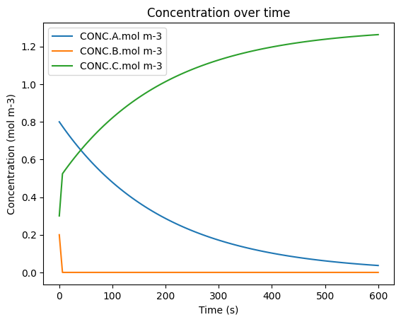
# Plot the species concentrations over time
df.plot(x='time.s', y=['CONC.A.mol m-3', 'CONC.B.mol m-3', 'CONC.C.mol m-3'],
        title='Concentration over time',
        ylabel='Concentration (mol m-3)',
        xlabel='Time (s)')
plt.show()

	time.s	ENV.temperature.K	ENV.pressure.Pa	ENV.air number density.mol m-3	CONC.A.mol m-3	CONC.B.mol m-3	CONC.C.mol m-3
0	0.0	200.0	70000.0	42.095324	0.800000	2.000000e-01	0.300000
1	6.0	200.0	70000.0	42.095324	0.775723	3.979221e-08	0.524277
2	12.0	200.0	70000.0	42.095324	0.752182	3.858465e-08	0.547818
3	18.0	200.0	70000.0	42.095324	0.729356	3.741374e-08	0.570644
4	24.0	200.0	70000.0	42.095324	0.707222	3.627836e-08	0.592777
...	...	...	...	...	...	...	...
96	576.0	200.0	70000.0	42.095324	0.041522	2.129939e-09	1.258478
97	582.0	200.0	70000.0	42.095324	0.040262	2.065302e-09	1.259738
98	588.0	200.0	70000.0	42.095324	0.039040	2.002627e-09	1.260960
99	594.0	200.0	70000.0	42.095324	0.037855	1.941854e-09	1.262145
100	600.0	200.0	70000.0	42.095324	0.036706	1.882926e-09	1.263294

101 rows × 7 columns

2. Loading a Custom JSON Box Model Configuration#

Loading your own JSON configuration file works the same way as loading a pre-made example. Simply provide the path to your custom configuration file instead of using the Examples class.

The example below loads a file called custom_box_model.json from the config subfolder:

[ ]:

from acom_music_box import MusicBox
import matplotlib.pyplot as plt
import logging
import sys

# Disable logging to reduce output noise
logging.disable(sys.maxsize)

# Create a MusicBox instance and load the custom configuration
box_model = MusicBox()
conditions_path = "config/custom_box_model.json"
box_model.loadJson(conditions_path)

# Solve the box model and display results
df = box_model.solve()
display(df)

# Plot the species concentrations over time
df.plot(x='time.s', y=['CONC.A.mol m-3', 'CONC.B.mol m-3', 'CONC.C.mol m-3'],
        title='Concentration over time',
        ylabel='Concentration (mol m-3)',
        xlabel='Time (s)')
plt.show()

Simulation Progress:   0%|          | 0/600.0 [00:00<?, ? [model integration steps (2.0 s)]/s]

	time.s	ENV.temperature.K	ENV.pressure.Pa	ENV.air number density.mol m-3	CONC.A.mol m-3	CONC.B.mol m-3	CONC.C.mol m-3
0	0.0	200.0	70000.0	42.095324	0.800000	2.000000e-01	0.300000
1	6.0	200.0	70000.0	42.095324	0.775723	3.979221e-08	0.524277
2	12.0	200.0	70000.0	42.095324	0.752182	3.858465e-08	0.547818
3	18.0	200.0	70000.0	42.095324	0.729356	3.741374e-08	0.570644
4	24.0	200.0	70000.0	42.095324	0.707222	3.627836e-08	0.592777
...	...	...	...	...	...	...	...
96	576.0	200.0	70000.0	42.095324	0.041522	2.129939e-09	1.258478
97	582.0	200.0	70000.0	42.095324	0.040262	2.065302e-09	1.259738
98	588.0	200.0	70000.0	42.095324	0.039040	2.002627e-09	1.260960
99	594.0	200.0	70000.0	42.095324	0.037855	1.941854e-09	1.262145
100	600.0	200.0	70000.0	42.095324	0.036706	1.882926e-09	1.263294

101 rows × 7 columns

Loading A Custom Box Model in MusicBox#

1. Loading Pre-made Box Model Examples#

2. Loading a Custom JSON Box Model Configuration#

This Page